SGD with Vanishing Correlated Gradient Errors

A common misconception

“More accurate gradient estimates must give a more precise final SGD estimate.”

This implication fails for online estimators that reuse historical data. Single-step errors shrink, but successive estimates repeatedly contain the same noise. These correlated errors accumulate in the Polyak–Ruppert (PR) average. Single-step MSE alone misses their effect across the optimization trajectory.

Model and common conditions

The question is concrete: an online gradient error bₜ vanishes, yet remains correlated across time because observations are reused. Does it affect convergence? Does it change the asymptotic variance of the averaged iterate?

• F: ℝᵖ → ℝ is differentiable, μ-strongly convex, and L-smooth, with 0 < μ ≤ L; θ* denotes its unique minimizer.
• The initial iterate satisfies E‖θ₁ − θ*‖² < ∞. The step size is ηₜ = Dt⁻α, with D > 0 and 1/2 < α < 1.
• For a filtration ℱₜ, θₜ, bₜ, and δₜ are ℱₜ-measurable; ξₜ₊₁ is ℱₜ₊₁-measurable and εₛ is ℱₛ-measurable. Wₜ,ₛ ∈ ℝᵖˣᑫ are deterministic matrices and εₛ ∈ ℝᑫ. Vector norms are Euclidean.

Theorem 1: convergence despite correlated errors

In addition to the common conditions, assume:

• The sampling noise is a martingale difference with bounded conditional second moment: almost surely, E[ξₜ₊₁ | ℱₜ] = 0 and E[‖ξₜ₊₁‖² | ℱₜ] ≤ σ² < ∞.
• The innovations εₛ are independent and centered, with a common finite covariance Q. Finite constants B_W, B_δ ≥ 0 satisfy the following bounds for every t ≥ 1:

Conclusion. Let aₜ = E‖θₜ − θ*‖². There exist finite constants C_init, C_ξ, C_b ≥ 0, c₀ > 0, and an integer n such that, for all t ≥ n:

Thus θₜ → θ* in mean square and almost surely. In fact, the conclusion only needs an adapted error satisfying E‖bₜ‖² ≤ B/t: bₜ need not be conditionally unbiased or independent across time.

What this resolves: Correlated, possibly biased online estimation errors do not prevent SGD from converging. Convergence, however, does not mean the final average has unchanged variance.

Theorem 2: what variance does PR averaging inherit?

Use the common conditions and the following complete additional assumptions; these replace, rather than inherit, Theorem 1’s noise assumptions:

• F is twice continuously differentiable, with H = ∇²F(θ*) ≻ 0. Its Hessian is globally Lipschitz: for a finite L_H ≥ 0, ‖∇²F(θ) − ∇²F(ϑ)‖op ≤ L_H‖θ − ϑ‖ for every θ, ϑ.
• The joint innovations Zₛ = (ξₛᵀ, εₛᵀ)ᵀ are i.i.d., centered, and have finite covariance. Write S = Cov(ξₛ), Q = Cov(εₛ), and C₀ = Cov(ξₛ, εₛ). Each Zₜ₊₁ is independent of ℱₜ. The two noise components may be correlated at the same time.
• For some B < ∞ and β > max{1/2, 2α − 1}, E‖bₜ‖² ≤ Bt⁻β for every t ≥ 1. The cumulative remainder T⁻¹ᐟ²∑ₜ₌₁ᵀ δₜ converges to zero in probability.
• Define cumulative weights K with first index T, the total horizon, and V_T as below. Require a covariance limit, an average-weight limit, and a maximal-weight condition:

Conclusion. For the average θ̄_T = T⁻¹∑ₜ₌₁ᵀ θₜ:

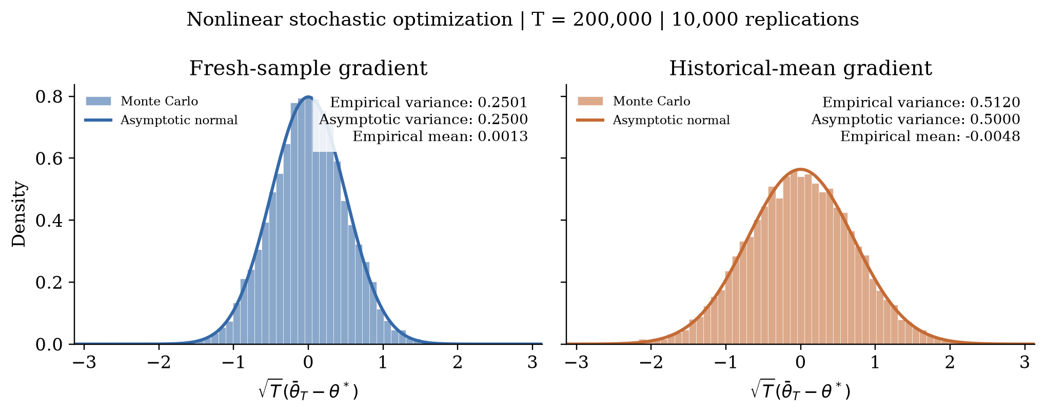
When C₀ = 0, the extra contribution is H⁻¹ΓH⁻ᵀ. Correlated noise components additionally require the cross terms. Γ comes from the historical weights; it also equals the limit of Cov(T⁻¹ᐟ²∑bₜ) if the cumulative remainder vanishes in L².

When can the errors be ignored? If β > 1, the other assumptions give the classical PR covariance H⁻¹SH⁻ᵀ without the three weight-limit conditions. β = 1 alone is insufficient: cumulative error covariance is bounded but need not converge. For 0 < β < 1, it may vanish, approach a nonzero finite limit, diverge, or remain bounded without converging.

What this resolves: “Gradient error vanishes” and “gradient error is negligible at the √T scale” are different requirements. The running mean has single-step error covariance Q/t, yet Γ = 2Q and therefore changes the PR limit.

Proposition 1: the variance bound for this estimator class

Conditions. The innovations εₛ ∈ ℝᵖ are i.i.d. and centered, with finite covariance Q. The scalar weights wₜ,ₛ are deterministic and sum to one at every step. Set bₜ = ∑ₛ₌₁ᵗ wₜ,ₛεₛ, with no additional remainder. Nonnegative weights are not required.

Let k(T,s) = ∑ₜ₌ₛᵀ wₜ,ₛ and Γ_T = Cov(T⁻¹ᐟ²∑ₜ₌₁ᵀ bₜ). For every T ≥ 1, the following identity holds:

Hence T⁻¹∑ₛ₌₁ᵀ(k(T,s) − 1)² → 0 implies Γ_T → Q; when Q ≠ 0, it is also necessary. If Theorem 2’s PR conditions hold, C₀ = 0, and Γ_T → Γ, then:

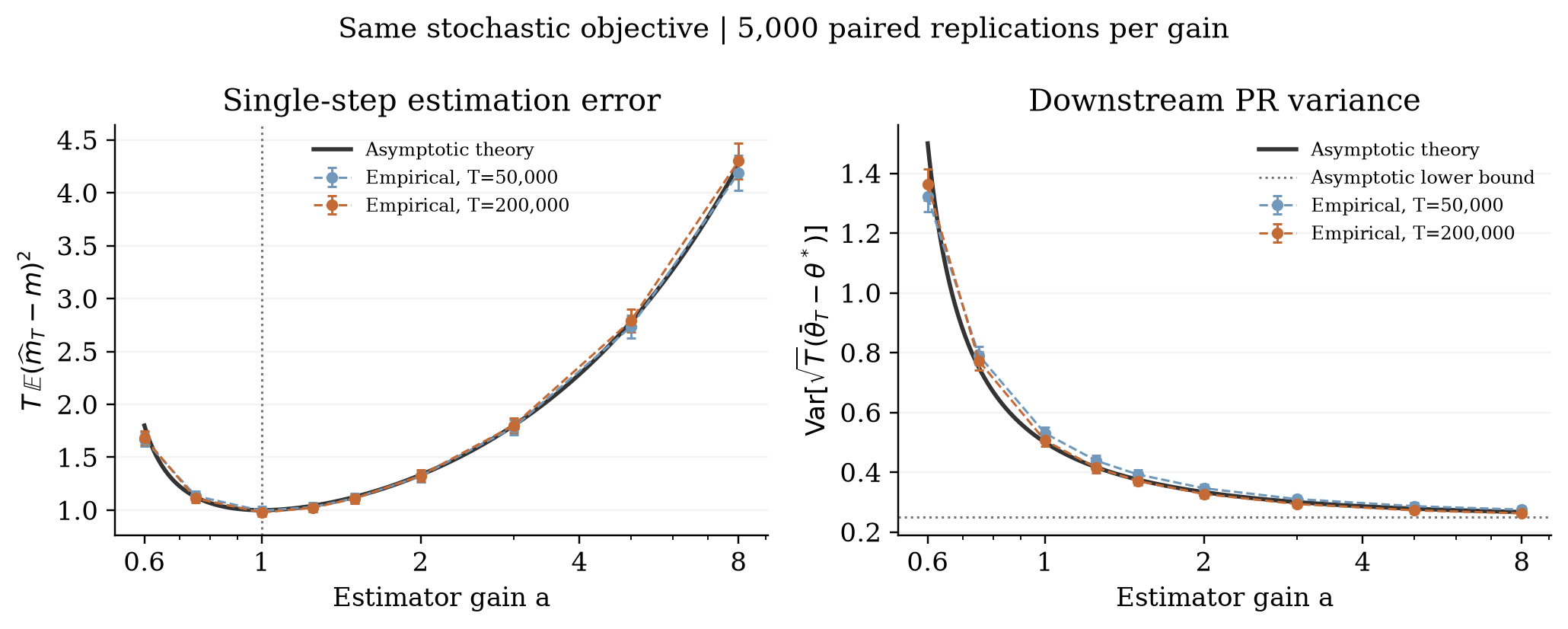
What this resolves: This normalized historical linear estimator class has an exact benchmark for final variance. The bound is specific to this class, rather than universal across stochastic optimization algorithms.

Proposition 2: slower single-step estimation can attain the bound

Conditions and construction. Use Proposition 1’s innovation assumptions. Choose 0 < a ≤ 1 and 1/2 < ρ < 1, initialize b₁ = ε₁, and then update:

The initialization ensures nonnegative, exactly normalized historical weights. The construction satisfies:

If Theorem 2’s objective, initial-iterate, step-size, and joint-innovation conditions also hold, C₀ = 0, and ρ > 2α − 1, the downstream PR covariance is exactly H⁻¹(S + Q)H⁻ᵀ, attaining Proposition 1’s bound.

What this resolves: The running mean has faster O(t⁻¹) single-step MSE but contributes 2Q. This construction has only O(t⁻ρ) single-step MSE, yet contributes Q. The relevant objective is the efficiency of the final estimate, rather than auxiliary single-step accuracy alone.