CCSGD · eggtea

Nonlinear-feature regression: parameter MSE for CCSGD and six baselines — **Nonlinear-feature regression.** Parameter MSE averaged over 256 paired runs. The fitted CCSGD slope is −0.978, consistent with O(t⁻¹). Dashed lines show the specified baselines’ asymptotic squared biases, not finite-time lower bounds.

Neural-network regression: clean-input prediction MSE for CCSGD and six baselines — **Neural-network regression.** Prediction MSE averaged over five paired runs; shading shows CCSGD’s empirical 20–80% quantiles. The plot ends at 1.1×10⁵ updates, where CCSGD is lower. At the full 2×10⁵ updates, CCSGD / SIMEX MSE is 0.0142 / 0.0125. Global growth control is not established for this network, so these curves are empirical results.

The algorithm: complex correction of noisy inputs

We want to minimize the expected loss F on clean inputs, but observe only W = Z + U. Evaluating gradients directly at W generally changes the objective. Let g be the loss gradient with respect to the real parameter θ, and gℂ its entire extension in the input.

F (θ) = 𝔼_{Z} ℓ (θ; Z), g (θ; z) = \nabla_{θ} ℓ (θ; z)

For Gaussian error U ∼ N(0, Ω) with known covariance Ω, take a fresh observation Wₜ and independently draw Vₜ ∼ N(0, Ω). Evaluate the full complex score at Wₜ + iVₜ, take its real part, and perform an ordinary SGD update. Ω may be singular and need not be diagonal.

G_{t} = Re g^{ℂ} (θ_{t}; W_{t} + i V_{t}), θ_{t + 1} = θ_{t} - η_{t} G_{t}

When a response Y is present, complexify only the input and keep the observed Y fixed. Use the analytic extension of the loss without introducing complex conjugation. Averaging several imaginary perturbations for one observation reduces simulation variance, while observation variability remains.

The core: exact unbiasedness, not a finite-order approximation

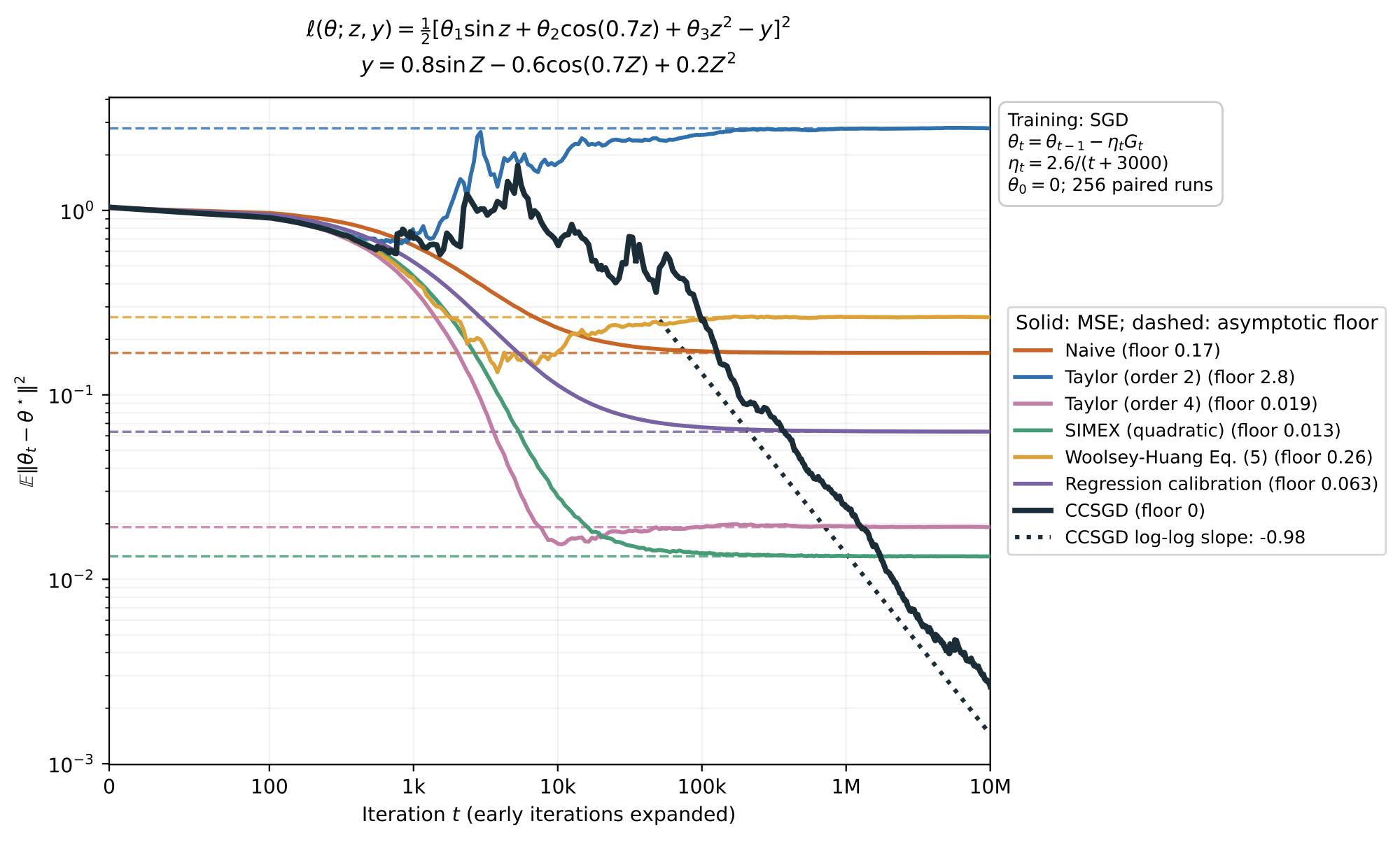
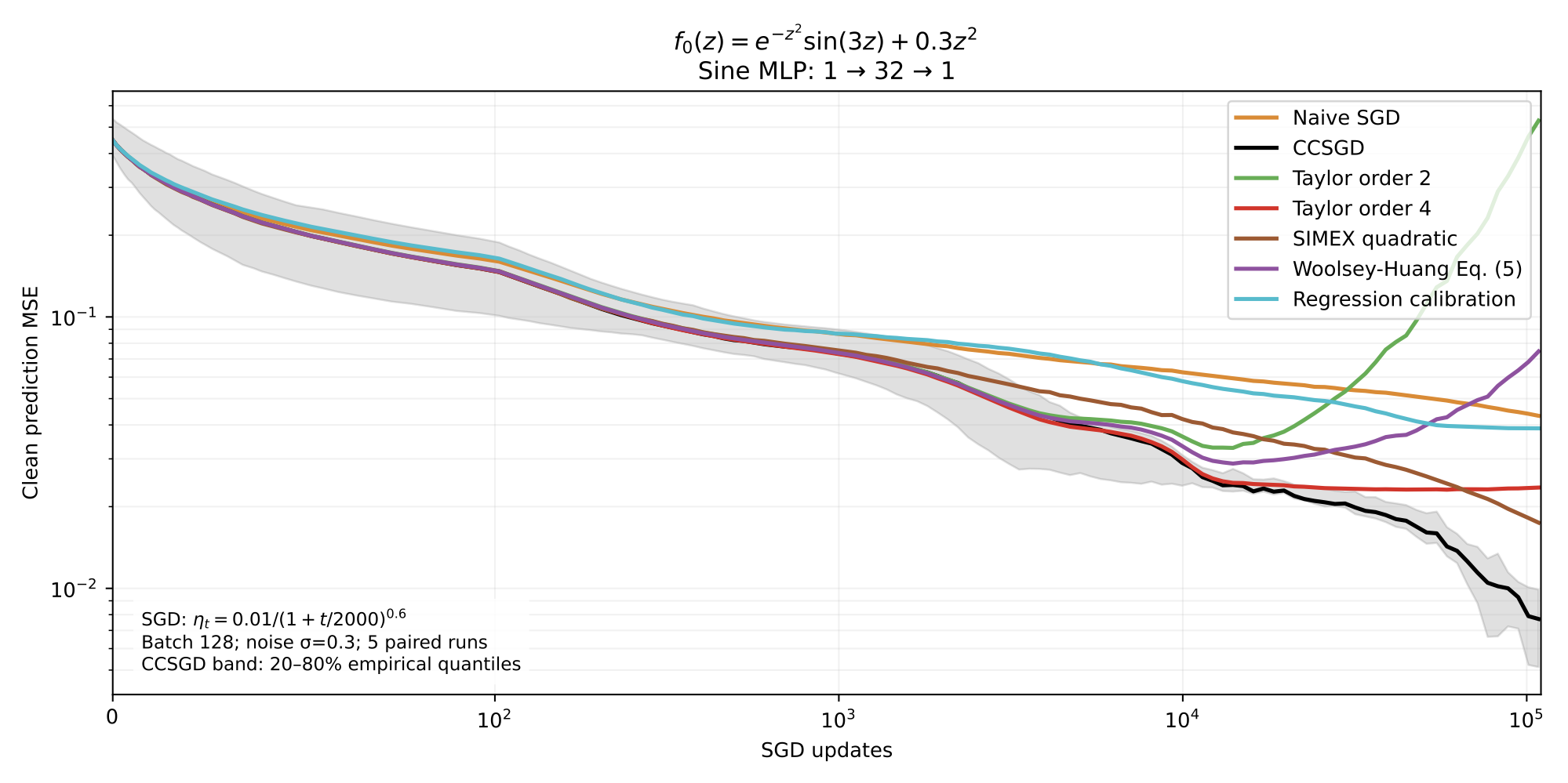
Under an entire extension and suitable growth and integrability conditions, the classical complex corrected-score identity recovers the clean score exactly: for each fixed (θ, z), average jointly over measurement error U and the independent perturbation V.

𝔼_{U, V} [Re g^{ℂ} (θ; z + U + i V)] = g (θ; z)

For independent scalar Gaussian U and V with the same variance, the exponential transforms of the real and imaginary perturbations cancel exactly:

𝔼 [e^{s (U + i V)}] = e^{\frac{σ^{2} s^{2}}{2}} e^{- \frac{σ^{2} s^{2}}{2}} = 1

Writing D = U + iV, all positive-order complex moments E[Dᵏ] vanish. Taylor expansion gives the identity below for polynomials; for entire functions, interchanging the sum and expectation requires integrability. “Exact” means all higher-order terms vanish in expectation, not that a single gradient evaluation is noise-free.

𝔼 [h (z + D)] = \sum_{k = 0}^{\infty} \frac{h^{(k)} (z)}{k!} 𝔼 [D^{k}] = h (z)

van Dantzig pairs: which errors admit this correction?

For general errors, the imaginary perturbation cannot be chosen arbitrarily. For symmetric scalar error U whose moment-generating function is finite on the real line, we seek an independent real V whose characteristic function is its reciprocal. This is the van Dantzig pair used here.

M_{U} (s) φ_{V} (s) = 1 \Leftrightarrow φ_{V} (s) = \frac{1}{M_{U} (s)}

Here Mᵤ(s) = E[exp(sU)] and φᵥ(s) = E[exp(isV)]. Such V exists exactly when 1/Mᵤ is a characteristic function; the companion paper develops Fourier and moment criteria and constructions. Gaussian error has a Gaussian conjugate of the same variance, but in general V has a different law from U.

U ∼ Unif[−b, b]: V is centered logistic with scale b/π.
P(U = ±b) = 1/2: V has density 1 / [2b cosh(πv/(2b))].

The pairing yields cancellation of complex moments. Exact correction for entire scores additionally requires Taylor integrability; SGD theory further needs second moments and appropriate growth control. The construction therefore applies to admissible pairs satisfying these conditions, rather than arbitrary noise.

Connecting the correction to classical SGD theory

Let ℱₜ₋₁ denote the past. With fresh samples independent of that past and differentiation interchangeable with expectation, the corrected score is conditionally unbiased for the clean objective:

𝔼 [G_{t} | ℱ_{t - 1}] = \nabla F (θ_{t})

Unbiasedness is the first step. The paper bounds input-derivative growth by ‖Dq gℂ(θ; q)‖ ≤ M(θ) exp(a‖q‖) with a parameter-independent exponent a, controls the parameter-dependent amplitude as below, and separately assumes a relative variance bound for the clean sample gradient.

{M (θ)}^{2} \leq A + B {‖ \nabla F (θ) ‖}^{2}

Together with sub-Gaussian latent inputs and suitable noise moments, these conditions derive the conditional variance structure used in classical stochastic approximation, rather than assuming it for the corrected score:

𝔼 [{‖ G_{t} - \nabla F (θ_{t}) ‖}^{2} | ℱ_{t - 1}] \leq σ^{2} + ρ {‖ \nabla F (θ_{t}) ‖}^{2}

Under the corresponding objective, step-size, and local regularity assumptions, standard SGD analysis then gives:

Convex, smooth objectives: objective-gap bounds for step-size-weighted averages.
Strongly convex, smooth objectives: almost-sure convergence and mean-square rates. With c/(t+γ)ᵅ and 1/2 < α < 1, the rate is O(t⁻ᵅ); at α = 1 it is O(t⁻¹) when 2μc > 1.
Smooth nonconvex objectives: bounds on weighted mean squared gradient norms, giving stationarity guarantees.
With additional local regularity and covariance conditions: central limit laws for the last iterate and Polyak–Ruppert averages, with a distinct averaging covariance at α = 1.

Correction restores the clean gradient in expectation. Measurement and simulation noise remain in the variance and asymptotic covariance. Non-Gaussian pairs must satisfy the corresponding moment conditions before these optimization conclusions transfer.

Read the full CCSGD paper ↗